By Sergey Tselovalnikov on 18 November 2020
Indirect Effects of Allocate Direct
Hi, folks!
Every single program allocates memory. Byte buffers are at the core of many essential libraries which power the services the modern internet is built upon. If you’re building such a library, or even just copying data between different files, chances are you’ll need to allocate a buffer.
In Java, ByteBuffer is the class that allows you to do so. Once you’ve
decided to allocate a buffer, you’ll be presented with two methods
allocate() and allocateDirect(). Which one to use? The answer is, as
always, it depends. If there were no tradeoffs, there wouldn’t be two
methods. In this article, I’ll explore some of these tradeoffs,
demystify this behaviour, and I hope that the answer will be clear for
you by the end of it.

Yeah well, sometimes the things we do don’t matter right now. Sometimes they matter later. We have to care more about later sometimes, you know.
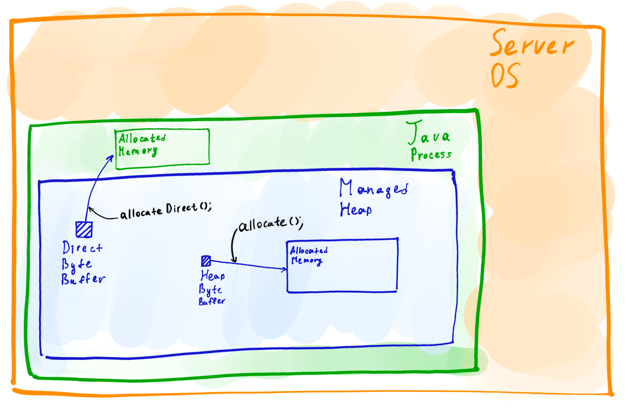
Two buffers
At first glance, the two methods allocate() and allocateDirect() are
very simple. The allocate() allocates a buffer in the managed heap of
the Java process, a part of this exact space which size is specified
with the Xmx option. The allocateDirect() method allocates a buffer
residing outside of the managed heap.
This difference, however, creates a number of significant runtime implications, which I’m going to dive into here. But first, let me start by telling a debugging story where direct byte buffers were the murderer.
The story
Every story needs a protagonist. In this case, the protagonist was a Java application built on top of RSocket, a modern application protocol. Here’s the oversimplified version of the app which you can find on Github. Let’s call this app an echo app. The echo code isn’t trying to do anything complicated, it is a simple echo service built with an awesome rsocket-java library. All it does is spins up a client and a server, where the client sends messages, and the server echoes them back.
var server = RSocketServer.create(echo) //...
var client = RSocketConnector.create() //...
while (true) {
  assert Objects.equals(client.send(), client.receive())
}
| ❗️ | The supporting code for this article is available on Github. You can, and I highly encourage you to, choose to go through each step yourself by cloning the code and running each example with a simple bash script. All measurements were taken on an EC2 AWS m5.large instance. Unless specified otherwise, Java 13 is used. The point of this article is not to show the numbers but rather demonstrate the techniques that you can use to debug your own application. |
|---|
The code is useless if it’s just sitting in the repo and doing nothing, so let’s clone the repo and start the app.
git clone https://github.com/SerCeMan/allocatedirect.git
cd allocatedirect && ./start.sh
The app starts, and you should see that the logs are flowing. As expected, now it’s processing a large number of messages. However, if the echo app was exposed to users, they would start noticing significant pauses every now and then. All Java developers know that the first thing to look at in the case of spurious pauses is GC.
| ❗️ | You can find GC logs of the app are stored in /tmp/${gcname}. The example logs for each run are also available in the repo. In this article, gceasy.io was used for visualisation. It’s a great free online tool which supports the log format of multiple garbage collectors. Even though you can always visualise GC logs using a tool like gceasy, as we’ll see later, the raw logs often contain a lot more information than most of the tools can display. |
|---|
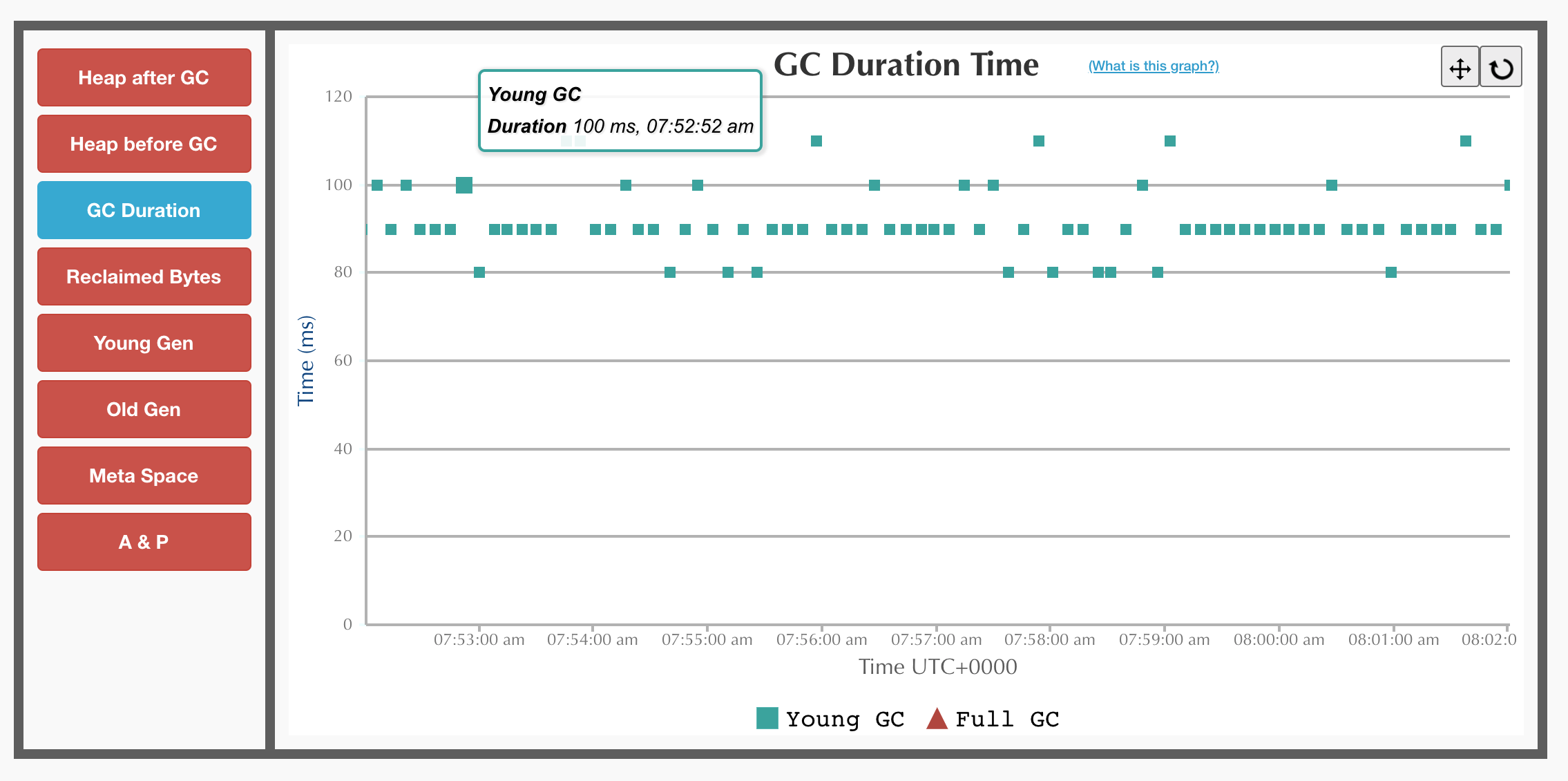
Indeed, GC logs show that GC is to blame here. The application is running under G1, which is the default collector since JDK 9. There are multiple young GC pauses on the graph. Young GC is a stop-the-world pause in GC in G1. The application stops completely to perform a cleanup. For the echo server, the graph shows multiple young GC pauses that last for 100-130ms and occur every 10 seconds.
G1 GC
Luckily for us, in the last few years, there has been an amazing development in the GC space. There are not just one but two new fully concurrent garbage collectors, ZGC and Shenandoah.
While I’ve had great success with ZGC before, Shenandoah has a great advantage of being much friendlier to application memory consumption. Many applications, especially simple JSON in, JSON out stateless services are not memory-constrained. Some application, on the other hand, especially the ones that process a large number of connections might be very sensitive to memory usage.
Even though the echo app only has a single client and a server in its current state, it could as well handle tens of thousands of connections. It’s time to enable Shenandoah, and run the echo app again.
./start.sh shen # starts with -XX:+UseShenandoahGC
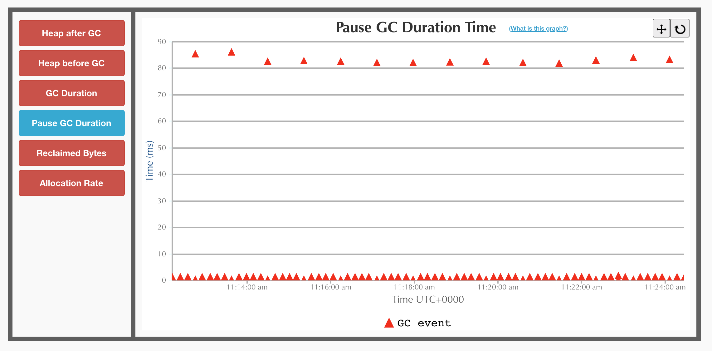
After enabling Shenandoah, the GC logs start showing an interesting picture. There is definitely a huge improvement in the pause frequency. The pauses now only occur every minute or so. However, the pauses are still around 90ms long, which is far away from the desired sub-millisecond pauses.
Shenandoah GC
Now that the symptoms are clear, and the problem is reproducible, it’s time to look at the cause. GC graphs don’t show much more information. Looking at the raw logs directly, on the other hand, reveals the cause which is clearly stated right on the pause line.
...
[info][gc] GC(15) Pause Final Mark (process weakrefs) 86.167ms
...
Turns out, weak references are to blame. Put simply, weak references are a way to keep an object in memory until there is a demand for this memory. Large in-memory caches is a common use-case for weak references. If there is enough free heap, a weak reference cache entry can stay there. As soon as GC figures out that there is not enough memory, it’ll deallocate weak references. In most of the cases, this is a much better outcome than the application failing with an out of memory exception because of a cache.
A frantic search across the repository doesn’t show any usages of weak, soft or phantom references. Not even the search through the third party libraries can show anything. After staring at the metrics for a while, one of the graphs gives a clue! The long GC pauses correlate with a sudden drop in the number of direct byte buffers.
GC vs DirectByteBuffer count
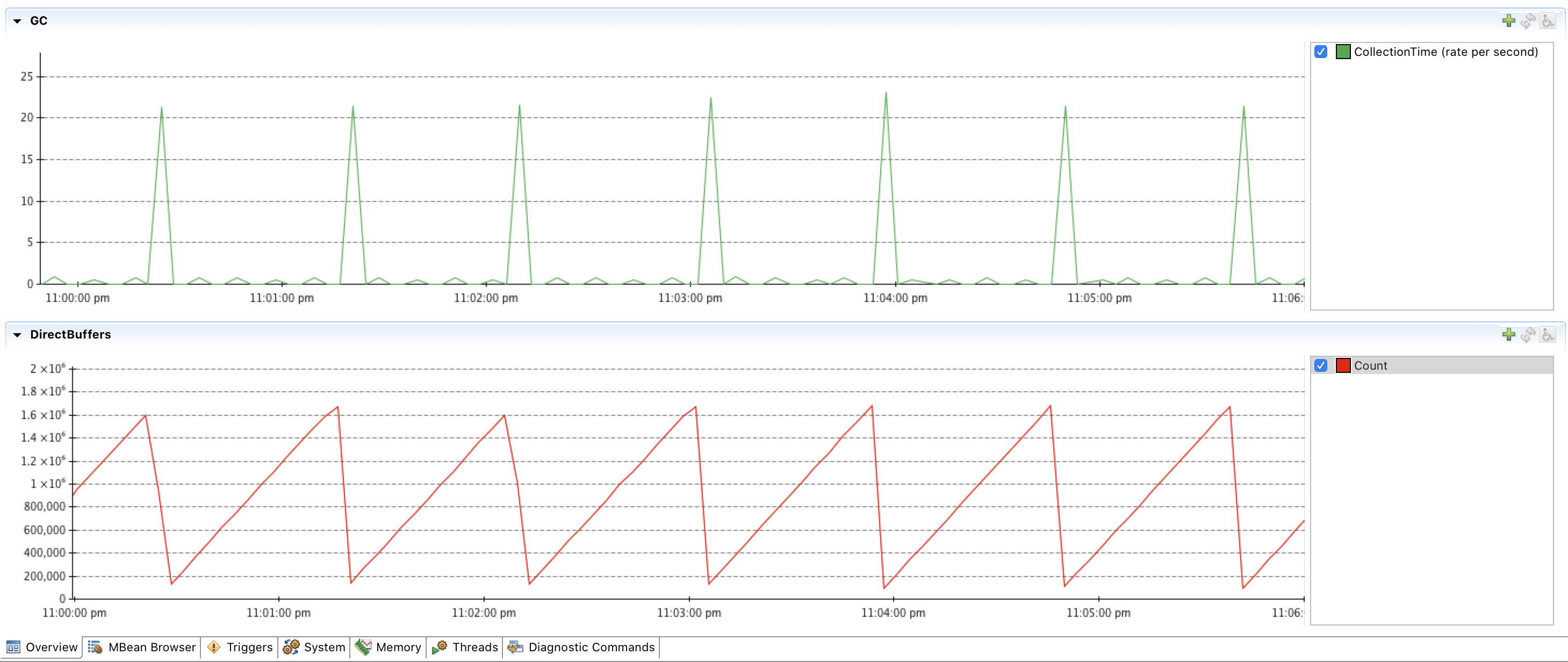
| ❗️ | You can get a similar graph by running the echo app and connecting to the JMX port. For this screenshot, I used Java Mission Control (JMC). The start.sh script contains the options that you can enable to connect to an app with JMX remotely. |
|---|
At first, the correlation might not make any sense. Byte buffers are not
weak references, are they? They are not weak references themselves.
However, you might notice, that creating a new direct byte buffer gives
you back a plain ByteBuffer interface which doesn’t have a close
method or any other way of deallocating the buffer.
ByteBuffer buf = ByteBuffer.allocateDirect(42);
The underlying buffer needs to go away once the last reference to this
buffer goes away. The modern API for this in Java is
java.lang.ref.Cleaner.
As we can see, it’s exactly what DirectByteBuffer class uses to
determine when the underlying buffer should be deallocated.
DirectByteBuffer constructor
DirectByteBuffer(int cap) {
    // ...
    base = UNSAFE.allocateMemory(size); // malloc call
    UNSAFE.setMemory(base, size, (byte) 0);
    // ...
    cleaner = Cleaner.create(this, new Deallocator(base, size, cap));
}
Yet, there are no usages of direct buffers in the code of the echo app either, so how could we find them? One way would be to search through the third party libraries using IntelliJ. The approach would work very well for the echo example but would completely fail for any real applications of a decent size. There are just way too many places where byte buffers are used. Looking at the graphs, one can notice that the number of created buffers per minute is huge, literally millions of them.
Instead of searching through the code to find all byte buffer
references, it is easier to find the place at runtime. One way to find
out where the majority of the buffers is created is to fire up the async
profiler and profile the
malloc calls
which are used by direct buffers to allocate memory.
# async profiler can be downloaded from https://github.com/jvm-profiling-tools/async-profiler
./profiler.sh -d 30 -f /tmp/flamegraph.svg $(pgrep -f java) -e malloc
While running, the profiler managed to sample more than 500000 malloc calls which non-ambiguously show where all of the buffers were created from.
malloc calls
| ❗️ | The flame graph above visualises the code paths where most of the captured malloc calls occur. The wider the column is, the larger the number of times the code path appeared in the sample. This graph, as well as other flame graphs in this article, is clickable. You can read more on how to read flame graphs here. |
|---|
As it turned out, there was a place in the code which was using direct
buffers. With this rich knowledge of where exactly the direct buffer
allocations occur, creating a fix is easy. All that’s needed is to make
a one line change and to replace allocateDirect with allocate and
send a PR upstream.
Running the same app on shenandoah after applying the single line change produces a completely different graph which pleases the eyes with sub-millisecond GC pauses.
Shenandoah GC
The costs
The story revealed a dark side of direct byte buffers. If there is a dark side, there must be a bright side as well! There is. But before we look at the bright side, we need to explore a few more sides which also appeared to be grey.
Allocations
Previously, we’ve observed implicit deallocations costs, so now it’s time to take a look at allocations. Could direct buffers be much cheaper to create? After all, going off-heap has been a performance trend for a while. A small benchmark can help to estimate the costs.
@Param({"128", "1024", "16384"})
int size;

@Benchmark
public ByteBuffer heap() {
  return ByteBuffer.allocate(size);
}

@Benchmark
public ByteBuffer direct() {
  return ByteBuffer.allocateDirect(size);
}
After cloning the repo, you can run the benchmark yourself with the command below.
# Don't just read! Clone the repo and try yourself! 🤓
./bench.sh alloc1
The absolute numbers are not that interesting. Even the slowest operation only takes a few microseconds. But the difference between the heap buffers and direct buffers is fascinating.
Benchmark               (size)  Mode  Cnt     Score     Error  Units
AllocateBuffer1.direct     128  avgt    5  1022.137 ± 148.510  ns/op
AllocateBuffer1.heap       128  avgt    5    23.969 ±   0.051  ns/op

AllocateBuffer1.direct    1024  avgt    5  1228.785 ± 127.090  ns/op
AllocateBuffer1.heap      1024  avgt    5   179.350 ±   2.989  ns/op

AllocateBuffer1.direct   16384  avgt    5  3039.485 ± 111.714  ns/op
AllocateBuffer1.heap     16384  avgt    5  2620.722 ±   5.395  ns/op
Even though direct buffers lose in all of the runs, the difference is much more noticeable on small buffers while on large buffers, the overhead is almost negligible. Due to the 50x difference on a small buffer, it’s a much more compelling example to look into. Let’s start a benchmark again, make it run for much longer, and use async profiler to see what where the time is spent.
ByteBuffer.allocateDirect()
The flame graph already hints towards some of the overhead. Not only the
direct buffers need to allocate memory, but it also needs to reserve it
to check the maximum native memory limit. On top of this, the buffer
needs to be zeroed as malloc can’t guarantee that it doesn’t return
you some garbage while the buffer needs to be ready to use. And finally,
it needs to register itself for deallocation as a soft reference. All of
this seems like a lot of work, but the actual allocation still takes a
half of the time! So, even if the heap buffer doesn’t need to do any
work other than calling malloc, it should only be as twice as slow,
not 50 times! Profiling heap buffer allocations can hopefully reveal
where such a vast difference is coming from.
ByteBuffer.allocate()
The heap buffer flame graph is surprisingly blank. There isn’t much
happening on the graph. Yet, there are still some allocations in the
yellow flame tower on the right. However, the whole allocation path only
takes 2% of the time, and the rest is nothing? Exploring the yellow
tower gives a further clue. Most of its time is taken by a function
that’s called MemAllocator::allocate_inside_tlab_slow. The meaning of
the allocate_slow part is self-explanatory, but it’s inside_tlab
that is the answer.
TLAB stands for Thread Local Allocation Buffer. TLAB is a space in the
Eden, the space where all new objects are born, dedicated for each
thread to allocate objects. When different threads allocate memory, they
don’t have to contend on the global memory. Every thread allocates
objects locally, and because the buffer is not shared with other
threads, there is no need to use call malloc. All that’s needed is to
move the pointer by a few bytes. The fact that most of the allocations
happen in TLAB could explain why heap buffers are so much faster when
their size is small. When the size is large, the allocations won’t occur
in TLAB due to the limits on its size, which will result in buffer
allocation times being almost on par.
Now that we’ve assumed that we know why it’s so much faster, can we jump to the next section? Not so fast!
So far, TLAB is just a theory, and we need to conduct an experiment to
validate it. One of the easiest ways is to simply disable TLAB with the
-XX:-UseTLAB options.
// run with ./bench.sh alloc4
@Fork(jvmArgsAppend = { "-XX:-UseTLAB" })
@Benchmark
public ByteBuffer heap() {
  return ByteBuffer.allocate(size);
}
Benchmark             (size)  Mode  Cnt    Score   Error  Units
AllocateBuffer2.heap     128  avgt    5  151.999 ± 8.477  ns/op
Were we right? Yes and no. The performance results with disabled TLAB
are not as impressive anymore. Though, the pure allocation time is still
about three times faster even considering that the benchmark needs to
not only allocate memory for the buffer itself but also for the
ByteBuffer class. The still significant difference shows the cost of
going back to the operating system with a syscall every time to ask for
more memory with occasional page faults.
ByteBuffer.allocate(), -XX:-UseTLAB
As a rule of thumb, if your buffers are mostly short-lived and small, using heap byte buffers will likely be a more performant choice for you. Conveniently, it’s exactly what the javadoc of the ByteBuffer class is warning us about.
It is therefore recommended that direct buffers be allocated primarily for large, long-lived buffers that are subject to the underlying system’s native I/O operations.
— ByteBuffer.java
Memory costs
So far, we’ve only been measuring allocations. Still, looking at the
flame graphs, we can also see the de-allocation path which is frequently
invoked by JMH that runs the benchmarks by explicitly invoking
System.gc()
and finalization before each iteration. That way, the previously
allocated buffers will be deallocated.
However, in the real applications, as we saw in the debugging story, we’re at a mercy of the GC to deallocate those buffers. In this case, the amount of memory consumed by the app might be hard to predict as it depends on the GC and how the GC behaves on this workload. For how long would the following code run?
public class HeapMemoryChaser {
  public static void main(String[] args) {
    while (true) {
      ByteBuffer.allocate(1024);
    }
  }
}
The code above contains an infinite loop, so you can say forever, and you will be completely right. There are no conditions, so there is nothing that can prevent the loop from running. Will this snippet run forever too?
public class DirectMemoryChaser {
  public static void main(String[] args) {
    while (true) {
      ByteBuffer.allocateDirect(1024);
    }
  }
}
Will the above code run forever as well? It depends on how lucky we are.
There are no guarantees on when a GC would clean up the allocated direct
buffers. Various JVM options can vary the result from run forever with
no issues to a crash after a few seconds. Running the above code with
-Xmx6G on a VM with 8GB RAM runs for about 20 seconds until it gets
killed by the operating system.
$ time java -Xmx6G DirectMemoryChaser
Killed

real    0m24.211s
dmesg shows an insightful message explaining that the process was
killed due to lack of memory.
[...] Out of memory: Killed process 4560 (java) total-vm:10119088kB, anon-rss:7624780kB, file-rss:1336kB, shmem-rss:0kB, UID:1000 pgtables:15216kB oom_score_adj:0
[...] oom_reaper: reaped process 4560 (java), now anon-rss:0kB, file-rss:0kB, shmem-rss:0kB
Allocating direct buffers without care can cause the app to go far beyond the expected memory usage as there are no guarantees on when the soft references are going to be cleaned. Crashing right after the start is counterintuitively a good result. At least, you can observe the failure, reproduce it, understand it and fix it. A crash after a few hours of running is much worse, and without a clear feedback loop, it’s much harder to resolve the issue.
When debugging such issues, or as a preventative measure, consider using
-XX:+AlwaysPreTouch to at least exclude the heap growth out of the
equation. One way to prevent this is to run the infinite growth of
direct buffers is to use -XX:MaxDirectMemorySize=${MAX_DIRECT_MEM} to
ensure that the usage of direct memory doesn’t grow uncontrollably.
The benefits
So far, the direct byte buffers have only caused troubles. In the story, switching to heap-based byte buffers was a clear win, though there are a lot of hidden dangers in using them. Would it be reasonable to use heap byte buffers only and never use direct buffers? The choice exists for a reason, and there reasons to use direct buffers.
Off Heap Graal
We have observed problems with allocations and deallocations, so what if
a buffer is only allocated once and never deallocated? One buffer is not
enough most of the time, so you can create a pool of buffers, borrow
them for some time and then return back. It is what Netty does with
their ByteBuf
classes which are built to fix some of the downsides of the ByteBuffer
class. Nevertheless, it’s still not clear why one should prefer direct
buffers over heap buffers.
Avoiding GC altogether could be one of the reason. You could be managing terabytes of memory without any GC overhead. While you could manage large amounts of memory with direct byte buffers, there is a limit of 2^31 on the indices that you can use with a single buffer. A solution is coming in the form of a Foreign-Memory Access API which is available for the second preview in JDK 15. But avoiding GC is not the main reason.
IO
The IO is where direct byte buffers shine! Let’s say we need to copy some memory between two files. Heap byte buffers are obviously backed by memory in a heap, so the contents of the files would have to be copied to be sent back seconds later. This can be avoided completely with direct byte buffers. Direct byte buffers excel when you don’t need a buffer per se but rather a pointer to a piece of memory somewhere outside of the heap. Again, at this point, this is only a hypothesis of a random person on the internet. Let’s prove or disprove it with the following benchmark.
@Benchmark // ./bench.sh reverse
public void reverseBytesInFiles() throws Exception {
  ByteBuffer buf = this.buffer;
  buf.clear();
  try (FileChannel channel1 = FileChannel.open(Paths.get(DIR + "file1"), READ);
       FileChannel channel2 = FileChannel.open(Paths.get(DIR + "file2"), WRITE)) {
    while (buf.hasRemaining()) {
      channel1.read(buf);
    }
    buf.put(0, buf.get(SIZE - 1));
    buf.flip();
    while (buf.hasRemaining()) {
      channel2.write(buf);
    }
  }
}
The code above reads 64 MB of random data from the first files, reverses
the byte order of each long in the array and then puts it back.
Reversing the first and the last bytes here is a tiny operation which
the only goal is to modify the contents of the file in some way as
copying could simply be done by calling channel.transferTo.
The results show that the direct buffer is the clear winner, almost twice as fast!
Benchmark                              (bufferType)  Mode  Cnt   Score   Error  Units
CopyFileBenchmark.reverseBytesInFiles        direct  avgt    5  36.383 ± 0.683  ms/op
CopyFileBenchmark.reverseBytesInFiles          heap  avgt    5  59.816 ± 0.834  ms/op
The next step is to understand where the time was spent to validate our hypothesis. Taking a flamegraph for the direct buffer shows what we expected — all of the time spent in kernel reading and writing files.
Directy Buffer
For the heap buffer, for both operations, reading and writing, the
memory has to be copied first between the buffers which we can clearly
see from the flamegraph. A solid chunk of it is taken by the
copyMemory function.
Heap Buffer
The IO here does not only refer to writing to disk, but it can also be writing to a socket which is what a considerable portion of the java applications is performing all day non-stop. As you can see, carefully choosing your buffers can significantly affect performance.
Endianness
Can direct byte buffers be even faster? While reading the javadoc for create methods, note an important remark:
The new buffer’s position will be zero, its limit will be its capacity, its mark will be undefined, each of its elements will be initialized to zero, and its byte order will be ByteOrder#BIG_ENDIAN.
— ByteBuffer.java
The byte order of byte buffers created in java is always big endian by
default. While having an always predictable default is great, it also
means that sometimes, it might not match the endianness of the
underlying platform. In the case of an m5.large AWS instance, this is
indeed the case.
jshell> java.nio.ByteOrder.nativeOrder()
$1 ==> LITTLE_ENDIAN
This fact immediately raises the question if, or rather when changing endianness can yield any significant performance wins. The only way to find out is to measure it.
static final int SIZE = 1024 * 1024 * 1024;

@Param({"direct-native-order", "direct"})
String bufferType;

@Setup
public void setUp() throws Exception {
  switch (bufferType) {
    case "direct":
      buffer = ByteBuffer.allocateDirect(SIZE); break;
    case "direct-native-order":
      buffer = ByteBuffer.allocateDirect(SIZE).order(ByteOrder.nativeOrder()); break;
  }
  channel = FileChannel.open(Paths.get("/dev/urandom"), READ);
  while (buffer.hasRemaining()) { channel.read(buffer); }
  buffer.flip();
  this.buffer = buffer.asLongBuffer();
}

@Benchmark // run with ./bench.sh order
public long sumBytes() {
  long sum = 0;
  for (int i = 0; i < SIZE / 8; i++) {
    sum += buffer.get(i);
  }
  return sum;
}
The above benchmark measures a specific use-case. We load a gigabyte worth of random longs into memory. Then, we simply read them one by one. It’s interesting that depending on the endianness, the result will be different as it affects the order of the bytes. We don’t care about the byte order for this use-case, however, as a random value with reversed byte order is still a random value.
Benchmark                       (bufferType)  Mode  Cnt    Score   Error  Units
OrderBenchmark.sumBytes  direct-native-order  avgt    5  136.025 ± 2.262  ms/op
OrderBenchmark.sumBytes               direct  avgt    5  195.980 ± 8.360  ms/op
The first impression is that iterating through a gigabyte worth of random memory is pretty darn fast. The second is that the native order byte buffer is performing 1.5 times faster! As before, running async profiler helps to reveal the reason why the native order is more performant.
Non-native (Big Endian)
Native (Little Endian)
Comparing the graphs above, the first difference that stands out is that
byte buffer classes are actually different depending on the byte order.
The native buffer is DirectLongBufferU while the non-native one is
DirectLongBufferS. The main difference between them is the presence of
the Bits.swap method.
Looking further into the method, we can see that it delegates directly
to Long.reverseBytes. While its implementation in Java is quite
complex, one can notice the @HotSpotIntrinsicCandidate annotation. The
annotation is a signal that at runtime, JIT could replace the method
with pre-prepared assembly code. Adding a set of JVM options,
-XX:CompileCommand=print,\*OrderBenchmark.sumBytes*, to the benchmark
allows us to peek at the resulting assembly code to understand how
exactly the reverseBytes affects the resulting code.
| Non-native (Big Endian) | Native (Little Endian) |
|---|---|
| |
Comparing the compilations listings of these two implementations, we can
notice that the biggest difference between them is the bswap
instruction which is the essence of the Bytes.swap method. As
expected, it reverses the byte order every time a long is read from the
buffer.
Reading a gigabyte of memory into longs is an interesting workload, but it’s not necessarily the one that you’re likely to encounter in production. Endianness can be a useful thing to remember about, but unless working with native libraries or working with massive files, it’s unlikely to be a concern.
Conclusion
Every non-trivial Java application directly or indirectly uses byte buffers. On the surface, ByteBuffer is a simple class. It’s just a pointer to a chunk of memory. Nevertheless, even by looking at such a simple class, you can discover a deep rabbit hole. Even though we’ve only looked at the tip of the iceberg, I hope that you have a clear idea now of when you could use a heap buffer, and when you would choose a direct buffer.
Modern JVM runtimes are complicated environments. While they provide sane defaults, they also present multiple options. The choice is always there, it’s up to you to make that choice, but it’s crucial to be aware of the consequences. Fortunatelly, JVM runtimes also come with a whole lot of various observability tools, JMX metrics, GC logs, profilers, and if you really want it’s not even that hard to look at the generated assembly code. Using techniques shown in this article, you can make a choice not for the workload of a guy from the internet, but for your workload, which can result in amazing results in production later. We have to care more about later sometimes, you know.
Thank you to
- Uri Baghin and Paul Tune for reviewing the article.
- You for reading the article.
References
- Async Profiler
- Beyond ByteBuffers by Brian Goetz
- GC Easy GC Analyser
- JVM Anatomy Quark #4: TLAB allocation
- Netty - One Framework to rule them all by Norman Maurer
- Netty’s ByteBuf API
Discuss on
Subscribe
I'll be sending an email every time I publish a new post.
Or, subscribe with RSS.